Monday, October 11, 2010
Cruise report is finally finalized
Hello again! I've been very busy after the cruise to catch up with various on-land activities, but Will and I finally managed to wrap up a cruise report for MGL1004. Post-cruise data analysis will soon begin...
Monday, September 13, 2010
Arriving in Honolulu soon
Well, it's hard to believe, but this nearly-never-ending cruise will be finally over in less than 9 hours. I went to bed early this evening, but couldn't sleep (because of being too excited?), so I decided to get up in the middle of the night. It's actually in the morning in the East Coast time, so maybe it's a good idea. I need to adjust my time zone anyway, so that I can get back to my normal teaching duty more easily.
We took a group photo the other day. Most of people shown in the picture are from the science party (only one from the Langseth crew), so this is just half the population on this research vessel (actually I noticed a few members of the science party are missing here; they were probably sleeping). We usually work in different places at different shifts, doing our own duties, and we rarely get together like this. So this picture is great because it vividly testifies that a research cruise like ours is supported by so many hard-working people.
 Though this cruise is going to end, we'll try to keep this blog active to post anything interesting we find during post-cruise data analysis or whatever we think it appropriate to post. We'll revisit Shatsky Rise in the spring of 2002, and you'll see posting from seas again.
Friday, September 10, 2010
The End is Nigh
Only a few more days remain in the long transit from Shatsky Rise to Honolulu. As we approach our MGL1004’s final destination, I have started to think about how I will enjoy becoming submersed in all the simply luxuries of civilization again. For example; being able to make a phone call whenever I chose and being able to chose what I want for dinner from the super market, just to name a few. It is easy to take such luxuries for granted while shore side, but life at sea helps develop a little greater sense of appreciation.
Life at sea has had its advantages though. As Jun mentioned, the scenery is gorgeous. Looking out upon a vast ocean gives you a new sense of space. Being able to see for miles in all directions, with no buildings, mountains, or trees to obstruct your view. While at sea I have found myself in the galley for hours, engaged in interesting conversations with people who have had many interesting experiences from sailing. This has helped me find a greater appreciation for the entertainment value of a good old fashion conversation. Finally, being at sea for so long and isolated, to some extent, from the rest of the world you learn something about yourself. How you handle certain situations that most people never experience in a lifetime.
Overall, my experience aboard the R/V Marcus G. Langseth, as a watchstander for the Shatsky Rise cruise, has been a positive one. I am very glad that I signed on and will take away a great deal of experience and appreciation for life at sea and seismic data acquisition. I am appreciative to all who have made this experience possible!
Thursday, September 9, 2010
The Sheltering Sky
 I asked watchstanders to post a blog on a daily basis, but as you've seen, they seem to be exhausted and are not posting as frequently as I'd like to see... It may be understandable because this cruise turned out to be unusually long; it's 60 days total, and this is by far the longest cruise I've been on (my previous record was 44 days). One of our graduate students, Duayne, told me this morning that he couldn't look at computer screen any more because he was sort of burned out. I found it interesting because I never get tired of working with computer...
As I wrote in my previous post, this cruise was a great success overall, and this is mainly brought by the professionalism of the Langseth crew, the Lamont science tech group, and the WHOI OBS team. Will and I did all the planning, but the actual implementation of the plan was done so gracefully by them, and there was literally nothing left for us to do (watchstanders worked hard during their watch under the supervision of the tech group, but the PIs just had to look at monitors). The chief science officer, Robert Steinhaus, originally came from the industry of exploration geophysics, and we all benefited from the high industry standard he brought to the vessel. Though I never worked in the oil industry, I somehow felt I was having a virtual experience of being a client from ExxonMobil.
We also had a good fortune of having nice weather throughout the cruise. One of major concerns we had before the cruise is that this survey area can sometimes be hit by wayward typhoons, but we didn't have any during this cruise. Actually, we had more than just nice weather. We had spectacularly calm seas on several occasions. The picture shown was taken in the morning of August 26, and you don't normally expect this kind of sea in the middle of the Pacific. That was simply gorgeous. Just imagine yourself sailing in the vast ocean filled with these colors... Now approaching the end of the cruise, I've started to regret not spending more time outside the lab. I was busy working on computer, and because we had so many days at seas, I thought I could see these things as many times as I want. Scientific problems in front of me seemed more important and urgent, but maybe I should've enjoyed the life at seas more. This reminds me of the following quote from one of my favorite movies, "The Sheltering Sky":
"Because we don't know when we will die, we get to think of life as an inexhaustible well, yet everything happens only a certain number of times, and a very small number, really. How many more times will you remember a certain afternoon of your childhood, some afternoon that's so deeply a part of your being that you can't even conceive of your life without it? Perhaps four or five times more, perhaps not even that. How many more times will you watch the full moon rise? Perhaps twenty. And yet it all seems limitless."
So, watchstanders, how many times did you see a spellbinding sunrise or sunset during this cruise? I hope you saw many.
Wednesday, September 8, 2010
Mission complete

As of September 3, 2010, our survey of Shatsky Rise was completed, and we started transit to Honolulu. Because of two medical diversions, we couldn't finish everything we planned, but given the science days we ended up with, what we were able to achieve can be called a great success. The following is the executive summary of the cruise report, which we are currently trying to write up before the end of the cruise:
"R/V Marcus G. Langseth MGL1004 formed the major data acquisition phase of the NSF-funded project, "Geophysical Constraints on Mechanisms of Ocean Plateau Formation from Shatsky Rise, Northwest Pacific" (OCE-0926611). Deciphering the origins of large oceanic plateaus is a critical element for understanding mantle dynamics and its relation to terrestrial magmatism, and Shatsky Rise was chosen as a high-priority target because it provides a unique tectonic setting to distinguish between various models proposed for the formation of oceanic plateaus. The purpose of this survey was to provide critical missing information on (1) the thickness, velocity structure, and composition of the Shatsky Rise crust, and (2) the history of magmatic emplacement and later tectonic development of the Rise. This was planned to be achieved by acquiring seismic data along two refraction lines over the Tamu Massif, which represents the early, most voluminous phase of the Rise construction, and over 3,000 km of reflection lines covering both the Tamu and Ori Massifs, the latter of which corresponds to the intermediate phase of the plateau evolution.
The cruise was unfortunately hampered by two medical diversions, which took ~16 days in total, and even with a seven-day extension provided by NSF, the survey had to be scaled down to focus on the southern part, leaving the northern part to be completed in another cruise tentatively scheduled for spring 2012. The southern part includes all of refraction lines (yellow lines in the map) and around 1800 km of reflection transects (red lines), all on the Tamu Massif. The work remaining to be done includes the rest of reflection transects (dotted red lines), which extend from the northern flank of the Tamu Massif to the center of the Ori Massif.
The Langseth fired over 47,000 shots from its 36-gun tuned airgun source into an array of seismic receivers: the Langseth's 6-km-long multichannel streamer and 28 Woods Hole Oceanographic Institution ocean-bottom seismometers (OBSs). As far as the southern part of the survey is concerned, the operational goals of the experiment were achieved in full. All of 28 OBSs deployed (shown as circles) were recovered successfully, and all instruments returned high-quality data. Multichannel seismic (MCS) profiling was also conducted with no major issues, yielding high-quality reflection data. Migrated brute stacks of all MCS lines were produced during the cruise, exhibiting intriguing intrabasement reflectors as well as revealing the true lateral extent of Shatsky Rise. OBS data show spectacular wide-angle refraction and reflection arrivals with the source-receiver distance often exceeding 200 km. The data collected during this experiment are sufficient to accurately determine the entire crustal structure of the Tamu Massif and will provide key information on the early magmatic construction of Shatsky Rise. By combining with future seismic data from the northern part of the survey, this information will provide an important tectonic framework for synthesizing existing geological, geophysical, and geochemical data and for resolving the formation mechanism of this large igneous province."
Monday, September 6, 2010
Back to Hawaii & other things on my mind
It's about a week to the end of the cruise. We picked up all the seismometers and are on our way back to Hawaii. Life on the langseth is a little less hectic now. I had a lot of fun retrieving the seismometers and speaking with Jimmy Elsenbeck on very interesting features of the device that make them withstand large pressures deep down at the bottom of the sea. Impressive devices they are. Sitting down there at the bottom of the sea, at about 5 km for the deepest deployment, the seismometers can withstand pressures as large as 7,000 lbs/sq in. To make that possible they have to be made of thick hard borosilicate glass, yet they float to the surface when remotely activated, despite their being denser than water. We can thank the principle of floatation for that. Just hollow out the insides, get enough air in ( I spare us the math) and we can define a dimension for neutral buoyancy. That's convenient.
I feel that the trip was auspicious despite the two unscheduled transits to Japan due to medical emergencies. For one, I got to participate in the first seismometer deployment. I also picked up the last seismometer. Good times I say. There is now no need to do long shifts. We are cruising at a steady speed of 11 knots towards Hawaii and should be on land in about 6 days. I hear I may get a little land disorientation. Just a little, though.
Life on the Langseth also has a new dimension to it. We have ping pong tournaments. Every one participates, and its fun. Unfortunately, I didn't make it to the finals on any of the games - singles or doubles. Some people are just way better than I am. I guess I'll focus on my soccer skills. Jun, was my favorite though. But one of the WHOI guys won the singles. I guess his eye hand coordination from picking up all those seismometers came in handy.
I look into my screen and I feel it can't be long now. We'll get to Hawaii soon. Not that I haven't enjoyed the trip, but I think I'm about done with the beautiful blue seas, the amazing rush of device deployment, and the tireless hours in the deep bowels of the cruise ship, Langseth. It's time to go home, feel the solid hard ground under my feet, touch the green grass, and take in the whole experience, again and again.
Friday, September 3, 2010
Marine Multi-channel Seismic Processing (part-3)
(6) NMO & further multiples removal
When the velocity model is ready to go, we can apply NMO to get the data further ready for stack (ProMAX module: Nromal Moveout Correction). But right here, we may have something more to do. That is to further remove multiples. Remember we have applied deconvolution to suppress when pre-process. But it does not often come up the result as good as we want. So at this point, we have the velocity model in hand, we have chance to remove multiples in further extent after NMO. Typically, we would like to employ inside mute, F-K filter or Radon filter to deal with marine seismic multiples. Read the materials about these two kinds of filters, select the proper paramters for the executive modules, then test and compare to find out the best result. Please be patient again, paramter test will need some time.
(7) Stack
When the data are done in CDP domain after applying NMO and filters for multiple removal, they are ready to stack. There is not much work to do except choosing the proper parameters for stack and wait for it done (ProMAX module: CDP/Enmble Stack). But before stack, remember to employ Bandpass Filter to remove the noise generated by the previous processing step, and maybe employ Automitical Gain Control to enhance the deeper reflectors (TBD). Because the multiple removal filter(s) would suppress the primaries signal at the same time. And then, we have to wait for the flow to execute and complete, which will take a long time when we have like 60000 CDPs to stack.
(8) Time migration
Comparing the stacked seismic section plot and the formal near-trace plot at the very beginning, we can easily find that the stacked one has much stronger and clearer signal on the plot, showing more geological details. However, we could still see some diffrations on the stacked plot, which are due to steep and dip change on topography or layering. So it is time to do the migration to correct them. We use Memory F-K Migration with the smoothed velocity model (relative to the velocity model we built up for stack) to make it happen. On the seismic image after migration, we can tell the difference apparently in the dip and steep areas in the seismic section. At this point, most of our work on marine multi-channel seismic data processing are done.
(9) SEG-Y Output & Print
Pick the one with the best effect after stack and migration, and output as a standard SEG-Y file. Then use GMT (command: pssegy) to make a postscript plot of the seismic section and print it out on a big piece of paper in moderate scale with proper vertical exaggeration. Now let the scienctist to tell the geological story when they are pointing at that big paper.
Wednesday, September 1, 2010
OBS Recovery!
Hello! Remember those seismometers we sent to the bottom of the ocean a little over a month ago? Well we are currently in the process of resurrecting them from the abyss and hopefully they are pregnant with scientifically illuminating data seismic data.
The OBS recovery process is fairly straightforward, consisting of a few steps. First we must navigate to the location above the instrument. Once we are on site, the OBS guys begin their dialog with the instrument via acoustics and send the instrument the release command. The OBS is anchored to the seafloor by a steel plate that is attached by a metal cable. When the release command is sent, an electric current is sent through the metal cable and it dissolves. The process that causes the cable to dissolve is known as electrolysis, which is a chemical reaction that occurs with the assistance of electrical current. After the OBS is liberated from its seafloor anchor, it begins its 70 meter per minute accent to the surface. Some of the OBSs are being recovered from depths just over 3,000 meters. From such depths, it takes the OBS around 45 minutes to float to the surface!

Once on the surface, we must gain a visual report of it, then navigate to its location. It is sometimes quite difficult to maneuver a ship as large as the R/V Langseth around in order to collect a relatively small OBS. Once we are next to the OBS, we hook it and haul it on board using the A-frame winch. The salt water is the washed off of the OBS and it is secured for transit to the next OBS site. We have been averaging about 3 hours per OBS recovery and it will take us roughly 2.5 days to recover them all.
The OBSs are then taken back to Woods Hole Oceanographic Institute in Massachusetts, where the data is extracted from the instrument, QCd, and processed.
Monday, August 30, 2010
Isotropic and anisotropic earth media in exploration geophysics
When we are doing exploration seismology, we take seismic wave equations as our theoretical base, and often we mention acoustic wave equation, elastic wave equations of isotropic media and anisotropic media. Real earth media should be considered as anisotropic media. VTI (transversely isotropic with vertical axis) media or TTI (transversely isotropic with tilted axis) media are the best approximation for complex geologic areas, while in relatively simple geological areas, all the seismic data processing steps can be taken under the assumption that the media are acoustic. This simplification has its reason that acoustic wave equation techniques are much mature than elastic (anisotropic, even isotropic) wave equation techniques. If we consider elastic wave equation, then we must deal with converted waves such like PP, PS, SP, SS, and so on, waves, which will add much difficulties for practical seismic data processing.
When we talk about elastic media, we want to differentiate different kinds of elastic media by their definite physical characteristics. Elasticity is one significant (almost most significant) character of elastic media. It is characterized by second rank elasticity tensor. According to elasticity theory, a second rank elasticity tensor has limited symmetries, and different symmetries will result in different types of earth models. In exploration seismology, elastic tensor is used in the form of its corresponding 6 by 6 elastic matrix because of its symmetries. There are the following kinds of anisotropic media, and at last the isotropic media can be considered as a special type of anisotropic media.
1. Generally anisotropic continuum has an elastic matrix that is symmetric and has 21 independent entries.
2. Monoclinic continuum is a continuum whose symmetry group contains a reflection about a plane through the origin. The elasticity matrix is also a symmetry matrix with 12 independent entries.
3. Orthotropic continuum is a continuum that possesses three orthogonal symmetry planes. The elasticity matrix has 9 independent entries.
4. Tetragonal continuum is a continuum whose symmetry group contains a four-fold rotation and a reflection through the plane that contains the axis of rotation. The elasticity matrix of tetragonal continuum has 6 independent entries.
5. Transversely isotropic continuum is a continuum that is invariant with respect to a single rotation. The elasticity matrix of transversely isotropic continuum has 5 independent parameters. Transversely isotropic media is a kind of very important media in exploration seismology and reservoir geophysics, since either VTI or TTI media can be considered as the approximation of real sedimentary geology, where the sedimentary layers lay parallel layer by layer.
6. Isotropic continuum is a continuum whose symmetry group contains all orthogonal transformations. Only two independent parameters are needed to describe the elasticity matrix of isotropic continuum. And sometimes people will conveniently use Lame parameters, which can be expressed as the linear combination of these two independent parameters, to solve problems.
Researchers are now using more and more anisotropic techniques to implement seismic data processing, since practical cases indicate that in some complex areas, anisotropy is necessary. However, anisotropic methods still have a lot of problems and is still under construction.
Sunday, August 29, 2010
More Crew Profiles
 1.Name/Title
-Nicky Applewhite/OS
2. Fave food/music/vacation destination
-Fried Chicken/R & B/Atlantic City
3. If you were stuck on a deserted island with only one person from this boat, who would you choose an
 d why?
-Dave DuBois (OBS) because he's a jokester
 1.Name/Title
-Rachel Widerman/3rd Mate
2. Fave food/music/constellation
Grilled Calamari/depends on my mood/Orion
3. If you were stuck on a deserted island with only one person from th
 is boat, who would you choose and why?
-Hervin because he's gonna cook and bring his ipod
 1.Name/Title
-Hervin Fuller/Steward
2. Fave food/music/kitchen utensil
-Italian/Opera/12 inch knife
3. If you were stuck on a deserted island with only one person from this boat, who would you choose and why?
 -Jason (Boson) because we like to hang out and we will be good at solving problems
 1.Name/Title
-Mike Tatro/Acquisition Leader
2. Fave food/music/tool
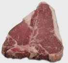
-Steak/Country/Monkey Wrench
3. If you were stuck on a deserted island with only one person from this boat, who would you choose and why?
-Ca
 rlos (Source Mechanic) because he's my fave
Friday, August 27, 2010
Marine Multi-channel Seismic Processing (part-2)
(4) Pre-process
With the raw shot data with geometry laoded, we are looking forward to seeing changes happen to make the data better till the final image of cross-section. The first thing we do is to use Ormsby bandpass filter to remove the noise generated during acquisition (ProMAX module: Bandpass Filter). Remember we have done the main frequency range analysis when we get raw shot data by using Interactive Spectral Analysis module. Take it and use it in bandpass filter. You can see big difference after employing this filter to the raw shot. The second thing we do is to edit the traces, including to kill bad channels (ProMAX module: Trace Kill/Reverse) and to remove the spikes and brusts (ProMAX module: Spike and Noise Edit). Remember we have known the bad channels using Trace Display when we just get the raw shot data in hand. So input the information in Trace Kill to get rid of those bad ones. All right, after these two steps, we have been able to see the difference from raw data. It is much better, isn't it?
But not good enough. The third thing we do in the pre-process is deconvolution. With the help of deconvolution, we could enhance the primaries and suppress the multiples (ProMAX module: Spking and Predictive Decon). Here, we need to test some critical parameters of the deconvolution, to figure out which ones create best results. It takes time! Please be patient, and read the related books and papers to understand how the deconvolution works and how it could work better.
(5) Velocity Analysis
After the pre-process flow, we have got better-look data in hand. It is time for us to do velocity analysis (ProMAX module: Velocity Analysis), which will take a lot time to complete. So be patient enough to get this step done. First of all, we start with large CDP interval, for example, 5000 CDP interval in a section of 60000 CDPs. When we conduct the velocity analysis, remember to use the near-trace plot that we have made before so that we could recognize the main horizons, and keep the direct wave, primaries and multiples paths in mind, so as to distinguish the primaries from multiples. Try our best to keep veolocity analysis away from multiples, and we know it is not always easy honestly.
Technically, we have stack velocity and interval velocity during velocity analysis, while stack one is lower than the interval one. However, we try our best to keep both of them increase reasonably with increasing depth. Because the seismic velocities of different layers or horizons will increase with depth in common cases due to the increase of some physical attributes like density. And the main factor for quality control during velocity analysis is to see the flat horizons after applying NMO (Normal Moveout). That is to say, if we pick the accurate velocity for the certain horizon, we are able to see the straight or flat coherent event in the trace gather. Sometimes we have some obvious coherent event to apply NMO to make sure the correct velocity we pick, especially in the upper layers, but sometimes not, especially in the lower layers. So in this unlucky situation, we would like to use the semblance graph to find out the energy concentration hotspot, and together with the increasing velocity with increasing depth in mind, to pick predictive velocities.
Again, be carefull of multiples. Because they will show up with hotspots in the semblance which might get you confused in some points, but the distinct thing is that they just have the same or similar velocity all the way down with the increasing depth, i.e., the multiples' velocity function curve should be a nearly straight line from the top down to the bottom. Anyway, try our best to be away from multiples during the whole process of velocity analysis. As long as we build up the brute velocity model with the large CDP interval, we can conduct the so-called brute stack. When we want to see more details for the strutures or something interesting, we need to denser the CDP interval for velocity analysis, for example, go for 2500 CDP, 1000 CDP interval, or even smaller CDP interval for some specific areas to image the relative smaller struture. So it depends on where is the interesting place we want to look at, how much details we want to see and what geolocial question we want to answer.
To Be Continued, see you next week, part 3!
Thursday, August 26, 2010
Give me the Earth, cut it up, and I'll give you a nautical mile!
We approached th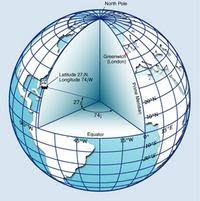 e centre of the rise today. There has not been a lot to do since we started collecting multi channel seismic data. Maybe when we start recovering the OBSs I'll get to go up to the deck more often. We did sight a pod of whales today, though. This was a first for me. The whales were far off so I couldn't make them out very well. All I saw was the jet of water they made ever so often. Apart from this exciting event all I have been doing during my watch is looking at the monitors, recording OBS crossings and thinking about how long it'd take to get to the next site. I keep asking myself, "How long will it take before I can take my eyes off the paper I'm reading and record the next crossing? "
I see now. The ship travels at 5 knots. The knot? A very convenient measure of "nautical"speed: 1 nautical mile per hour. Nautical, anything relating to navigation. We navigate on the seas. The Earth. The distances make sense. 1 nautical mile ~ 2 kilometers ~ 1.2 miles. I am thinking to myself. If I run at my average running pace - I do have a best time, but Nike plus tells me I run ~ 9' 30''/ mile - how long will it take me to run round the world? I do the math. There are (360 * 60) nautical miles to run. Those miles give ~ ( 360 * 60 * 1.2) US miles. At my average running pace it'd take me ~ 237, 000 minutes. That's ~ 5 months and 12 days. I think I'll put off running round the world. Its a long night. I'm done with my watch and I want to return to bed, but I begin thinking about why we have to cut the earth into 360 parts. why 360 and 60? I am sure there are interesting reasons.
e centre of the rise today. There has not been a lot to do since we started collecting multi channel seismic data. Maybe when we start recovering the OBSs I'll get to go up to the deck more often. We did sight a pod of whales today, though. This was a first for me. The whales were far off so I couldn't make them out very well. All I saw was the jet of water they made ever so often. Apart from this exciting event all I have been doing during my watch is looking at the monitors, recording OBS crossings and thinking about how long it'd take to get to the next site. I keep asking myself, "How long will it take before I can take my eyes off the paper I'm reading and record the next crossing? "
But things are different on the Langseth. I am used to working with distances in kilometers, I am Nigerian and we inherited the British system. Now I get to the United States and I have learnt to intuit the Mile. I run in miles, I drive in miles, Google navigator feeds me distances in miles. I get it. Now I have to get used to two new units, distance in "nautical miles" and speed in "knots". That's how sailors of old measured distances and speed, and although we have distance conversions, we still measure speed in knots on this research vessel. So I try to dig out conversions, run a couple of google searches, and voila! I discover very interesting history on the definition of the distance. I learnt during my search that both units of distance, the nautical mile and the kilometer were both defined based on the Earth. The nautical mile is actually an English system and the meter was defined by the French. The nautical mile you get if you cut up the earth in half at the equator and divide the circumference of the circle you get into 360 degrees, then each degree into 60 minutes. A minute of arc will then be 1 nautical mile. Same thing for the kilometer: you cut up the Earth. This time you cut it from the North pole, make it pass through paris (for historical reasons) and then measure the distance from the North pole to the equator, divide by 10,000 and you get 1 kilometer.
I see now. The ship travels at 5 knots. The knot? A very convenient measure of "nautical"speed: 1 nautical mile per hour. Nautical, anything relating to navigation. We navigate on the seas. The Earth. The distances make sense. 1 nautical mile ~ 2 kilometers ~ 1.2 miles. I am thinking to myself. If I run at my average running pace - I do have a best time, but Nike plus tells me I run ~ 9' 30''/ mile - how long will it take me to run round the world? I do the math. There
are (360 * 60) nautical miles to run. Those miles give ~ ( 360 * 60 * 1.2) US miles. At my average running pace it'd take me ~ 237, 000 minutes. That's ~ 5 months and 12 days. I think I'll put off running round the world. Its a long night. I'm done with my watch and I want to return to bed, but I begin thinking about why we have to cut the earth into 360 parts. why 360 and 60? I am sure there are interesting reasons.
Wednesday, August 25, 2010
A Brief History of Our Understanding of Planet Earth.
We know surprisingly little about our planet! The reason for this is that we are not able to probe the depths of Earth directly and explore. Also, because geological processes occur on much longer timescales than humans are familiar in dealing with. What little that we do know, we learned in the past couple decades! We learned how to split the atom before we learned how our own planet worked. Here I provide a brief history of our journey in understanding our home, planet Earth.
The age of Earth was of scientific speculation for many centuries. Finally, in 1953, Clair Patterson at the University of Chicago determined the now accepted age of Earth of 4,550 million (plus or minus 70 million) years old. He accomplished this through the Uranium/Lead dating of meteorites, which are the building blocks of planets. But once we discovered how old Earth was, a significant question came into the scientific forefront. If Earth is in fact ancient, then where were all the ancient rocks?
It took quite some time to answer this question. But it all started a few years earlier with Alfred Wegner, a German Meteorologist from the University of Marburg. Wegner developed a theory to explain geologic anomalies such as similar rocks and fossils being located on the East coast of the U.S. and the North West coast of Africa. His theory was that Earth’s continents had once been connected together, in a large landmass known as Pangea, and had since split apart into their contemporary locations. This theory opened up another question, what sort of force could cause the continents to move and plow through the Earth’s crust?
In 1944, Arthur Holmes, an English geologist, published his text Principles of Physical Geology in which he laid out his “Continental Drift” theory, which described how convection currents inside Earth could be the forcing behind the continent’s motion. Many members of the scientific community still could not accept this as a viable explanation for the movement of continents.
At the time, many thought that the seafloor of Earth’s oceans was young and mucky from all the sediment that was eroded off the continents and washed down river into the oceans. During the Second World War, a mineralogist from Princeton, Harry Hess, was on board the USS Cape Johnson. On board the Johnson there was a new depth sounder called the fathomer that was made to aid in shallow water maneuvering. Hess realized the scientific potential of this device and never turned it off. Hess surprisingly found that the sea floor was not shallow and covered with sediment! It was in fact deep and scored everywhere with canyons, trenches, etc. This was indeed a surprising and exciting discovery.
In the 1950’s oceanographers found the largest and most extensive mountain range on Earth, in the middle of the Atlantic Ocean. The mountain range, known as the Mid-Atlantic Ridge, was very interesting, being that it seemed to run exactly down the middle of the ocean and had a large canyon running down the middle of it. In the 1960’s, core samples showed that the seafloor was young at the ridge and got progressively older with distance away from the ridge. Harry Hess considered this and came to the conclusion that new crust was being formed at the ridge and was being pushed away from it as new crust came along behind it. The process became known as seafloor spreading.
It was later discovered that where the oceanic crust met continental crust, the oceanic crust subsided underneath the continental crust and sank into the interior of the planet. These were called subduction zones and their presence was able to explain where all the sediment had gone (back into the interior of the planet) and the youthful age of the seafloor (the older portion of seafloor currently being around 175 million years old at the Marianas Trench).
The term “Continental Drift” was then discarded, once it was realized that the entire crust moved and not just the continents. Various names were used to refer to the giant separate chunks of crust, including “Crustal Blocks,” and “Paving Stone.” In 1968, three American seismologists in the paper in the Journal of Geophysical Research called the chunks “Plates,” and coined the name for the science that we still use today, “Plate Tectonics.”
Finally it all made sense! Plate tectonics were the surface manifestation of convection currents in Earth’s mantle. This explained where all the ancient rocks on Earth’s surface went, that they were recycled back into the interior of the Earth. Plate tectonics gave answers to many questions in geology, and Earth made a lot more sense.
Plate tectonics are the surface manifestation of convection currents in Earth’s mantle. Convection involves upwellings and downwellings like in a boiling pot of water. Subduction zones are the downwellings in Earth’s convection system. Upwellings known as plumes are thought to exist, where hot material rises to the surface of the planet from the very hot interior. These plumes are thought to cause volcanism at the surface that are known as Large Igneous Provinces, such as the Shatsky Rise. We are out here today, continuing our journey of learning and understanding how our planet works. The data collected during this survey will hopefully shed light on what processes produced that Shatsky Rise, and if it was in fact a plume from Earth’s interior.
Note: Most of the information in this blog can be found in Bill Bryson's book, A Brief History of Nearly Everything
Monday, August 23, 2010
Anatomy of an Airgun
So far most of the talks have been an introduction to what we do, but little respect has b een paid as to how we do it. Therefor, today I will discuss the not so humble air gun.The gun pictured at right is not of our guns but of a single gun to give you an idea. We use an air gun array composed of 40 guns (similar to the one at right), 36 of which fire in tandem while 4 are left on standby. The total capacity of the array when operating at maximum is 6600 cubic inches of air. The remaining four guns are used in situations where we lose power to any of the other guns. However, there is a catch. The system cannot exceed 6600 cubic inches and each of the four standby guns weigh in at a hefty 180 cubic inches each. The largest guns are 360 cubic inches and the smallest are 60. So if a 60 goes out, we stop sending air to it, but if a 360 goes out we turn on two of the standby's to bring the volume back to 6600.
een paid as to how we do it. Therefor, today I will discuss the not so humble air gun.The gun pictured at right is not of our guns but of a single gun to give you an idea. We use an air gun array composed of 40 guns (similar to the one at right), 36 of which fire in tandem while 4 are left on standby. The total capacity of the array when operating at maximum is 6600 cubic inches of air. The remaining four guns are used in situations where we lose power to any of the other guns. However, there is a catch. The system cannot exceed 6600 cubic inches and each of the four standby guns weigh in at a hefty 180 cubic inches each. The largest guns are 360 cubic inches and the smallest are 60. So if a 60 goes out, we stop sending air to it, but if a 360 goes out we turn on two of the standby's to bring the volume back to 6600.If you need a rough approximation of what 6600 cubic inches pressurized to 2000 psi of air exploding is like, imagine that a standard SCUBA tank is pressurized to 3000 psi and is roughly 80 cubic feet at one atmosphere of pressure 80 cubic feet = 138240 cubic inches. 6600 cu in * 2000 psi = 1.1*10^6 ft lbs of force. The SCUBA tank if it explodes would be 138240 * 3000 = 3.456*10^7 ft lbs of force. The SCUBA tank is an order of magnitude larger, however this does not take away from the power of the air guns. Think of the tank as a bomb whereas the air guns are a controlled source. Regardless of the reference the air guns are still dangerous and they are kept at 2000 psi almost at all times. This requires one powerful air compressor. We refill the air guns every 20s (or 50m whichever comes first), so we need a large volume compressor to basically instantaneously fill the guns to be ready to fire for the next shot. If we were using the volume of the SCUBA tank we would need a compressor that was an order of magnitude greater in volume output and 1.5 times more powerful. The point is, is this is not JAWS and we do not condone exploding SCUBA tanks as our source material.

The air guns are relatively deep penetration sources, operating at 100 to about 1200 Hz, to identify subsurfacegeologic layers and define the subsurface structure. In studies that require less resolution but substantial penetration, the air gun is usually preferable as compared to a water gun, because it is far more efficient at producing low frequency energy. It can be used in fresh or brackish (less saline) water found in lacustrine and estuarine environments. Both air guns (and water guns) can be used in shallow w
ater surveys and relatively deeper water environments, achieving resolution on the order of 10 to 15 meters and up to 2000 meters penetration. With proper tuning, the air guns work well in a wide variety of bottom types. Minimum operating water depths of about 10 meters are possible in acoustically “soft” bottoms. In areas with acoustically hard bottoms, deeper water depths of operation are required. The harder bottoms produce multiples, unwanted reflective energy that travels repeatedly between the sea surface and the sea floor or shallow-subsurface and obscures the desired primary reflected energy arrivals.
The air gun requires an air compressor on board the ship. For maximum resolution, the smallest chamber size is used. If maximum penetration is the goal, a larger chamber is configured, but resolution is lessened. Both guns have a stable and repeatable pulse in terms of frequency composition and amplitude and can be tuned to optimize the source signature.Air guns generate more signal strength than boomer, and sparker, and chirp systems. The air gun is towed astern. The return signals are received by a towed hydrophone array.
This post has been updated. The volume for the guns was misunderstood. The current post reflects the changes.
Migration in seismic data processing
By using OBSs and streamer, we can get seismic data. The next step is seismic data processing, which is in fact the central step for our mission. Among the many steps in seismic data processing, migration is considered as the critical part, which in fact determines the quality of the seismic data processing.
What is migration? Concisely, migration is the step that “moves” seismic data received at the surface receivers to a subsurface image, which is considered to be able to describe the structural information of subsurface. Migration is not the first child of seismic data processing. It was born only after 1930s and emerges rapidly after 1960s and 1970s with the development of digital wave-equation technique. Here I only give some brief description on modern depth migration methods and their comparison. For a more detailed chronology of seismic migration and imaging, please refer to A brief history of seismic migration by J. Bee Bednar on Geophysics Vol. 70, NO. 3, and please refer to An overview of depth imaging in exploration geophysics by John Etgen et al. on Geophysics Vol. 74, No.6, for a detailed description of modern depth imaging methods.
Basically there are two major classes of migration methods, ray-based migration and wave-equation migration. Ray-based migration is based on the high-frequency asymptotic solution of the wave-equation. So from its nature, ray-based migration is in fact wave-equation migration, however in practice, we still differentiate it from wave-equation migration, since they just follow a much different methodology when doing migration. Two main methods are included in ray-based migration, Kirchhoff migration and beam migration. Kirchhoff migration dominates the petroleum industry from 1980s to 1990s, and now is still a living method both in practice and in theoretical research. Kirchhoff migration has its advantages of great flexibility and small computing amount. However, as the Kirchhoff migration is based on ray-tracing, there are deadly limitations in its imaging ability, the most obvious of which is that it uses single arrives along single raypaths to reconstruct the entire wavefield. Beam migration mainly denotes the Gaussian-beam migration, which uses “fat” rays and they can overlap each other. Another important feature of beam migration is that they are not dip-limited. But again, as beam migration is based on rays, in they may fail to image correctly in complex geological areas. Wave-equation migration are based on either acoustic wave equation, which is based on the assumption that our earth is fluid, or elastic wave equation, which is based on the assumption that our earth should be considered to be elastic solid. There are one-way and two-way wave-equation migrations. One-way wave-equation migration (OWEM) applies Green identity, which expresses the wavefield at certain time by the wavefield at earlier time or later time. One-way wave equation downward-propagates the wavefields from zero depth and suffers no upward-propagating wavefields, which justifies “one-way”. By one-way wave equation, based on the separation of two-way wave equation, the source and receiver wavefields are downward extrapolated from shallower depth to deeper depth step by step, and then applying imaging conditions, we can get the migrated image of subsurface. There are mainly four methods to do the downward extrapolation: implicit finite-difference algorithms, which express the single square-root one-way wave equation with infinite fractional series (and truncated to be finite in practice) to numerically implement; stabilized explicit extrapolation methods, which designs numerically Green functions to downward-propagate the one-way wavefield; phase-shift propagation with multireference velocities; dual-space (space-wavenumber) methods, including split-step Fourier (SSF) migration, Fourier finite-difference (FFD) migration, phase-screen and generalized-screen methods, etc.. As its nature is the approximation to two-way wave-equation, OWEM suffers from dip-angle limitation, which means that they are difficult to image steep dips and may give poor reconstructed image in geologically complex areas. On the contrary, two-way wave-equation uses not Green identity but full wavefield to reconstruct the subsurface image. When we refer to two-way wave-equation migration, we often denote the reverse-time migration (RTM). There is no high-frequency assumption and dip-angle limitation in RTM since it uses full wave equation and propagates the wavefield in all directions. For prestack RTM, we implement it by forward-propagating the source wavefield in time and backward-propagate the receiver wavefield in time, and then we get the subsurface image by doing the wavefield crosscorrelation of the source and receiver wavefields. At the emergence of RTM in 1980s, it was almost abandoned because of its high computation cost, both in time consumption and in storage requirements. However in recent years, with the development of computing hardware and algorithms, such as PC cluster, parallel computing technique, GPGPU computing technique, and improvements in computing storage, RTM is gaining the popularity both in practice and theoretical research. In fact, RTM is the most accurate algorithm we can find at present to render a complete and reliable image of subsurface structures. From the beginning acoustic RTM, to recent anisotropic RTM, the RTM is becoming more and more powerful and more and more companies are using RTM as their primary choice.
Full-waveform inversion is another emerging technique for seismic imaging and inversion. But there are many unresolved problems in it. We do not give introduction here.
Saturday, August 21, 2010
Marine Multi-channel Seismic Data Processing (part-1)
I think it is time for ProMAX right now. What is ProMAX? It is a software package of Lankmark Graphics Corporation since 1989 of Halliburton, for processing reflection seismic data. It is commonly used in the energy industry. Is it free? Unfortunately not! Even kind of expensive when comparing to other programs that will do the same sort of thing like SIOSEIS. Also another unfriendly thing for ProMAX may be that it runs on flavors of UNIX like Red Hat (but note that: not all the UNIX system can make ProMAX work), and I guest most people would like Windows-based program, because they hate command lines and writing script! But the good thing is, ProMAX is a program of user interface! No writing script. Gi'gem! You just need to start ProMAX in the terminal, and then you will use the program as friendly as Windows.
OK, let us get down to the technical business. What we are doing for processing the marine relection seismic data on the boat are following some workflows:
(1) SEG-D data input
When we get the raw shot data tape by tape from the recording system on the seismic boat, they are in SEG-D format and every .RAW file stored in the tape stands for one single shot gather (one shot point with 468 channels & traces). We probably get 3 tapes of raw shot gathers per day, which are about 18 GB each with maximum 1273 .RAW files in one single full tape. Even we have SEG-D data immediately when the boat is investigating, but we do not have much things to do until we finish the whole single seismic line, because we need the processed navigation file in .p190 format to set up the geometry for following processing work, and the .p190 files just can provided at least after completing one whole seismic line (sometimes after several short lines they process several .p190s together to save money on the use of lisence of the program). However, we still have things to do: we could take a first look at the raw shot gathers (ProMAX module: Trace Display), to find out the overall situation including direct wave path, reflected ray path including primaries and multiples, noise and bad channels; we can also figure out the main frequency range (PromMAX module: Interactive Spectral Analysis); and we could also make a near-trace plot by only using the near group of every shot to show the first glimpse of geology. We can have a first basic look at the major horizons like sediment layers, transition layers, volcanic layers or acoustic basement. Scientists are willing to see the seismic image as soon as possible. So the near-trace plot is a good thing to show them to release their desire in real time.
(picture below: near-trace plot of MGL1004 MCS line A)

(2) Set up Geometry
When we get the .p190 files for the seismic lines, we are ready to start the whole process flow. The first thing we need to do is to set up the geometry (ProMAX module: 2D Marine Geometry Spreadsheet). A lot of information we need to provide to ProMAX: group interval(12.5m), shot interval(50m), sail line azimuth, source depth(9m), streamer depth(9m), shot point number, source location (easting-X and northing-Y), field file ID, water depth, date, time, near channel number(468), far channel number(1), minmum offset, maximum offset, CDP interval(6.25m), full fold number(59), etc. Anyway, a lot! It takes some time to fill out the sheet and we need to be careful to make sure all the information matching up together. Sometimes it will be tricky, so double check, even triple check!
(3) Load Geometry
When the geometry set-up or the Spreadsheet is done, we can load the geometry in the raw shot data (ProMAX module: Inline Geometry Header Load). It takes time! Remember every tape is 18 GB. It will take almost one hour for loading one tape in (maybe faster using better workstation). After loading all the tapes or all the raw shot SEG-D files in the ProMAX with the geometry, they are ready to go to the real part of processing. Hold on for a second. I say "real" here, because I mean we are starting to polish the raw data, i.e., where change happens!
 (picture on the left: ProMAX geometry assignment map)
To Be Continued, next week, part-2!
Friday, August 20, 2010
Saving 1,522 lives on the Titanic with technology from the Langseth: fact or fiction?
 My girlfriend once asked me a question a while ago, "why do you study ancient volcanism?" I must admit I found it a little difficult communicating in clear and simple terms the motive behind what I do. " I want to know why Earth works the way it does," I remember explaining. I also tried justifying my interest in using computers to investigate the earth: " You know, developments in existing seismic methods borrow from the fields of mathematics and medical imaging. Who knows, methods developed in this research may someday be used in other fields." I still convince myself that this is true. In reality, most scientists just love asking "why?" and sometimes we get amazing answers that lead to enormous technological benefits, most of which were not planned in the first place. This is a story of how technology in use on the Langseth inherits a lot from the curiosity and dedication of scientists who asked "why?" Oh! and how things may have been different on the Titanic with these technologies.
I start with three names. Two are popular, the last maybe not so. They are Albert Einstein, Leonardo da Vinci and Isidor Rabi. I mention their names because they were pioneers, and their curiosity and research lead to 3 important technologies. Everyone knows Einstein. He is reputably the most influential and greatest scientist that ever lived. To him we owe the theories of general and special relativity. It was because Einstein asked the question "What is gravity?" that led Isidor Rabi and others to pioneer work on developing the atomic clock. In our attempt to understand the atomic world, scientist successfully built highly accurate clocks. These clocks are fundamental to the functioning of the Global Positioning System or GPS.
Isidor Rabi is not so well known, but this doesn't make his contribution less important. He pioneered work on building accurate atomic clocks. And then there is Leonardo da Vinci. He is more famous for the Mona Lisa, but he was also a scientist and inventor, and to him the field of acoustics owes the experimentalists curiosity on the behavior of sound waves.
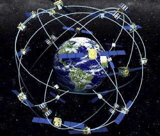 It was Leonardo da Vinci, as early as 1490, who first observed : “If you cause your ship to stop and place the head of a long tube in the water and place the outer extremity to your ear, you will hear ships at a great distance from you.” So pioneering the basis of acoustic methods. Duayne and Kai have shown how the Langseth conducts seismic experiments with sound sources. Acoustic methods are also used by marine mammal observers (MMOs) to listen to aquatic life. With the sound sources, accurate positioning made available by GPS, and the theory of sound, we can image Earth's interior. See the connection? Curiosity encapsulated in scientific endevour is the seed of technology. With this technology we can do better science, and also we reap enormous social benefits.
But I still haven't explained the Titanic connection. Yes, I'll admit it, I put in the Titanic connection to get the reader to follow me to the end of this post. But truthfully, let's revisit the history. Apart from the hubris of the engineers, at least that's what the movie Titanic suggests, could our application of science have saved the 1, 522 people who perished on board the titanic? Arguably so. Ten years following the tragedy, the Submarine Signal company of Boston commenced work on developing sonar devices to prevent such navigation hazards. And actually the first of these devices in the United States in 1914 by Reginald A. Fessenden. So with sound sources we could actually have prevented the disaster, and with GPS we could have very easily located the Titanic and saved more lives. Fact or Fiction? Fact!
Thursday, August 19, 2010
Crew Profiles
Hello all! As promised earlier, I now present you with mini interviews I conducted with various crew members. It takes copious amounts of work to keep this ship up and running so it seems only proper to introduce the hard working people that provide a safe and efficient means of data acquisition to science parties. I asked each person 3 main questions and here's what they had to say:
 1. Name/Title
-David Ng/Systems Analyst/Programmer

2. Favorite food/music/operating system
-Lobster/Rap and R&B/Ubuntu
3. You're stuck on a deserted island with only one person from this boat, who would you choose and why?
-Mik e Duffy because he can cook
1. Name/Title
-Robert Steinhaus/Chief Science Officer
2. Favorite food/music/science
-Mac & Cheese/Classic Rock/ Marine Seismic
3. You're stuck on a deserted island with only one person from this boat, who would you choose and why?
-Captai n Landow because people would look for him
1. Name/Title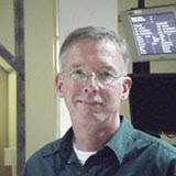
-Sir David Martinson/Chief Navigation
2. Favorite food/music/port
-Steak/Jazz/Aberdeen, Scotland
3. You're stuck on a deserted island with only one person from this boat, who would you choose and why?
-Pe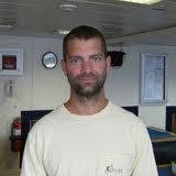 te (1st Engineer) because he can build and fix anything
1. Na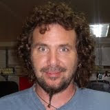 me/Title
-Bern McKiernan/Chief Acquisition
2. Favorite food/music/tool
-Animal/Mosh-pit music/Leatherman
3. You're stuck on a deserted island with only one person from this boat, who would you choose and why?
-Jason (Boatswain) because he's fun and handy with a small boat
More to come next week!!!!!
 1. Name/Title
-David Ng/Systems Analyst/Programmer

2. Favorite food/music/operating system
-Lobster/Rap and R&B/Ubuntu
3. You're stuck on a deserted island with only one person from this boat, who would you choose and why?
-Mik
 e Duffy because he can cook
1. Name/Title
-Robert Steinhaus/Chief Science Officer

2. Favorite food/music/science
-Mac & Cheese/Classic Rock/ Marine Seismic
3. You're stuck on a deserted island with only one person from this boat, who would you choose and why?
-Captai
 n Landow because people would look for him
1. Name/Title

-Sir David Martinson/Chief Navigation

2. Favorite food/music/port
-Steak/Jazz/Aberdeen, Scotland
3. You're stuck on a deserted island with only one person from this boat, who would you choose and why?
-Pe
 te (1st Engineer) because he can build and fix anything
1. Na
 me/Title
-Bern McKiernan/Chief Acquisition

2. Favorite food/music/tool
-Animal/Mosh-pit music/Leatherman
3. You're stuck on a deserted island with only one person from this boat, who would you choose and why?
-Jason
 (Boatswain) because he's fun and handy with a small boat
More to come next week!!!!!
Seismic Refraction and Reflection
Today I am going to explain the nature of seismic reflection and refraction and then briefly how we use it to extract information pertaining to the structure of Earth's subsurface. Let me start of with explaining what seismic refraction is.

The speed at which a seismic wave travels through a particular material is strongly dependent on the density and elastic properties of that material. So seismic waves travel at different speeds through materials with different properties. Generally, the denser the material, the faster seismic waves travel through it. When a seismic wave travels from one material into another, it does not continue in the same direction, but will bend. This bending of the seismic wave path is known as seismic refraction. Seismic refraction is caused by the difference in seismic wave speed between the two materials and is characterized by Snell’s Law, which is illustrated in the figure to the right. Given an angle of incidence (the angle between approaching seismic wave path and the line perpendicular to the interface) and the seismic wave speed in each material, Snell’s Law dictates the angle of refraction (the angle between the departing seismic wave path the line perpendicular to the interface).
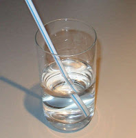
All waves(light, sound, etc.) undergo refraction when moving from one material to another. A good everyday example of refraction is when you look at a straw in a glass of water and the straw seems to bend where it enters the water. Well the straw is not actually bending but the path of the light traveling to your eyes from the submerged straw bends slightly as it enters the air from the water. This is because light travels at slightly different speeds through water and through air. It is this refraction (bending) of the path of the light from water to air that makes it appear that the straw is bent.

Now that we know what seismic refraction is, what is seismic reflection? The answer is that seismic reflection is a type of seismic refraction! When a seismic wave is travelling from a material with a lower seismic wave speed to a material with a higher seismic wave speed, the angle of refraction is larger than the angle of incidence. In this case, there exists an angle of incidence, where the angle of refraction is 90 degrees and the refracted seismic wave runs parallel to the interface between the two materials. The angle of incidence at which this occurs is known as the critical angle. When the angle of incidence is larger than the critical angle, the seismic wave is refracted back into material 1 and leaves the interface at the same angle as the incident seismic wave approached it. This post-critical refraction is call total internal reflection. These phenomena are illustrated in the figure just above, where the red wave path is critically refracted and the yellow wave path is reflected.
So how do we use seismic reflection and refraction to extract information about the structure of Earth’s subsurface? In general the density of material increases with depth in Earth, therefore the seismic wave speed increases with depth. As seismic waves travel down through the subsurface, they will see larger and larger velocity materials the deeper they go and according to Snell’s Law, will refract and reflect back up to the surface, where we can record them. Well by using controlled seismic sources (like the airguns described in Kai’s post) we can send seismic waves into Earth’s subsurface and record the reflections and refractions when the arrive. By measuring when these refractions and reflections arrive, we can determine where the interfaces between differing materials are in the subsurface, thus generating a cross-sectional view of the subsurface.
Subscribe to:
Posts (Atom)